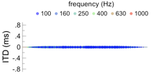
Acoustic cross-correlation or cross-covariance models measure left-ear and right-ear waveform similarity as a function of interaural time difference (ITD). Contributions to spatial hearing are then assumed to be the greatest from ITDs congruent with correlation maxima, indicating moments when the two waveforms were most similar.
The model performs well when representing ITDs under ideal listening conditions or when considering binaural signals exemplary of ideal listening conditions. In the examples below, for instance, ITDs with minimal fluctuations are imposed on nine noise-bursts: -0.8, -0.6, -0.4, -0.2, 0.0, 0.2, 0.4, 0.6 or 0.8 ms.
The cross-correlation model becomes less tenable under typical listening conditions, or when considering binaural signals exemplary of typical listening conditions. The first issue is that the model omits a strategy for interpreting sub-maximal correlations values indicating dissimilar waveforms and moments when ITDs are broadly distributed over time. The second, related, issue is that a verbatim interpretation of correlation values is inconsistent with psychoacoustic studies. Correlation values may remain low, for instance, when spatial cues fluctuate and are broadly distributed over time. Yet studies demonstrate that auditory images typically split into two distinct images (or two distinct ‘edges’) when distributions of spatial cues are broad enough. In the examples below, for instance, five ‘independence indices’ ranging from 1 to 0 are considered, where an index of 1 indicates that the waveforms in the left and right ears are statistically independent and an index of 0 indicates that the waveforms are identical.
Another issue for the cross-correlation model is when signal polarity or phase is inverted so that high correlation values are congruent with peripheral ITDs. Specifically, if intermediate correlation values (~0.0) prompt listeners to report split auditory images (or images with split edges), what should listeners report when when signal polarity is inverted? In the examples below, for instance, five ‘independence indices’ ranging from 0 to 1 are again considered when signal polarity was inverted.
Under the cross-correlation model, inverted correlations should, presumably, prompt listeners to report hearing two distinct images (or distinct edges) even more frequently than they do for intermediate correlation values (~0.0). Listening to signals exemplary of such conditions, however, demonstrates the opposite. Spatial hearing certainly broadens when signal polarity is inverted, yet images are considerably less broad (more compact) in comparison to when different noises are played in the ears causing spatial cues to fluctuate. Inverting polarity also results in a less definitive splitting of a single auditory image into two or more distinct images (or edges).
Pros:
• Cross-correlation procedures are easy to code and available for most software packages.
Cons:
- • Noise-bursts were 1 second long before passing through a bank of logarithmically spaced auditory filters.
- • ‘Fast’ cross-covariance was computed using the discrete Fourier transformation (DFT).
- • Correlations are normalized so that values range between -1 and 1.


